Numerical differentiation with a single function evaluation
Table of Contents
- Introduction
- Background
- The Problem
- Roundoff Error and Catastrophic Cancellation
- Complex Step Differentiation
Introduction
In this article, we’ll review complex step differentiation, a cool and perhaps little known technique for numerical differentiation that provides much greater accuracy than the popular finite difference based approaches. As the name suggests, this technique involves a little bit of complex analysis. However, we don’t expect any background and will try to keep this article fairly self-contained. If you’re anxious to know the technique, feel free to skip ahead. Otherwise, keep reading!
Background
Let’s start by reviewing the use of finite differences for numerical differentiation.
First-Order Approximations
Recall that the derivative \(f^{'}(x)\) of a function \(f: \mathbb{R} \to \mathbb{R}\) is defined as
\[f^{'}(x) = \lim_{h \to 0} \frac{f(x + h) - f(x)}{h}.\]Thus,
\[\frac{f(x + h) - f(x)}{h}\]is an approximation to the derivative \(f^{'}(x)\) which improves as \(h \to 0\). We can quantify the relationship between \(h\) and the error of the approximation using Taylor’s Theorem.
Taylor's Theorem
Let \( f: \mathbb{R} \to \mathbb{R} \), \( n \in \mathbb{Z}^+ \), and \( a \in \mathbb{R} \). Suppose \( f \) has \( n + 1 \) continuous derivatives on an open interval containing \( a \). Then, $$ f(x) = P_n(x) + R _{n + 1}(x)$$ where the \(n\)-th order Taylor polynomial $$P_n(x) = \sum _{k = 0}^{n} \frac{f^{(k)}(a)}{k!}(x - a)^{k}$$ and the remainder term $$R _{n + 1}(x) = \frac{f^{(n + 1)}(\xi)}{(n + 1)!}(x - a)^{n + 1}$$ for some \( \xi \) between \( a \) and \( x \).
Specifically, consider a 1st order Taylor polynomial centered at \(x\) and evaluated at \(x + h\), so that
\[f(x + h) = f(x) + hf^{'}(x) + h^2 \frac{f^{''}(\xi)}{2}\]for some \(\xi \in [x, x + h]\). Rearranging,
\[f^{'}(x) = \frac{f(x + h) - f(x)}{h} - \underbrace{h\frac{f^{''}(\xi)}{2}}_{\text{truncation error}}.\]Therefore, if \(f^{''}(x)\) is bounded then the truncation error (also called discretization error) of this scheme is \(O(h)\), making it a first-order method. The approximation
\[f^{'}(x) \approx \frac{f(x + h) - f(x)}{h}\]is known as the forward difference. Similarly, taking a Taylor polynomial centered at \(x\) and evaluated at \(x - h\), we recover the backward difference
\[f^{'}(x) \approx \frac{f(x) - f(x - h)}{h}\]which is also a first-order method. These are termed the one-sided formulas.
Higher-Order Approximations
We can obtain higher-order approximations to \(f^{'}\) by combining different Taylor expansions. For example, subtracting the expansions
\[\begin{align} f(x + h) &= f(x) + hf^{'}(x) + h^2\frac{f^{''}(x)}{2} + h^3 \frac{f^{(3)}(\xi_1)}{6} \quad\quad \xi_1 \in [x, x + h]\\ f(x - h) &= f(x) - hf^{'}(x) + h^2\frac{f^{''}(x)}{2} - h^3 \frac{f^{(3)}(\xi_2)}{6} \quad\quad \xi_2 \in [x - h, x] \end{align}\]we have
\[f(x + h) - f(x - h) = 2hf^{'}(x) + h^3 \frac{f^{(3)}(\xi_1) + f^{(3)}(\xi_2)}{6}\]and so
\[f^{'}(x) = \frac{f(x + h) - f(x - h)}{2h} - h^2 \frac{f^{(3)}(\xi_1) + f^{(3)}(\xi_2)}{12}.\]By the intermediate value theorem, there exists \(\xi \in [x - h, x + h]\) such that
\[f^{(3)}(\xi) = \frac{f^{(3)}(\xi_1) + f^{(3)}(\xi_2)}{2}\]and so
\[f^{'}(x) = \frac{f(x + h) - f(x - h)}{2h} - h^2 \frac{f^{(3)}(\xi)}{6}.\]Therefore, the approximation
\[f^{'}(x) \approx \frac{f(x + h) - f(x - h)}{2h}\]is second-order, i.e. \(O(h^2)\). It’s called the centered difference. You might see it equivalently written
\[f^{'}(x) \approx \frac{f(x + \frac{h}{2}) - f(x - \frac{h}{2})}{h}.\]Some Comments
From this analysis, it may seem that we’d always prefer the centered difference over the first-order methods because of the additional order in accuracy. However, there are instances where we’d choose a first-order method instead. For example:
- If \(f\) is expensive to compute, and we already know or have invested resources in computing \(f(x)\), then the first-order methods allow us to approximate the derivative with only one more function evaluation.
- If \(f\) is being evaluated at or near a singularity, the higher-order derivative present in the truncation error associated with centered difference can become intolerably large.
- If we’re evaluating \(f\) over a time series, and need the derivative at the current time, then we’d use a backward difference.
- When applied to initial-value (ordinary / partial / stochastic) differential equation problems, these schemes can have very different properties, which will not be covered here.
- If a function is evaluated over a grid of points (as done in various finite difference methods), you may require forward or backward difference at the boundaries of the grid.
The Problem
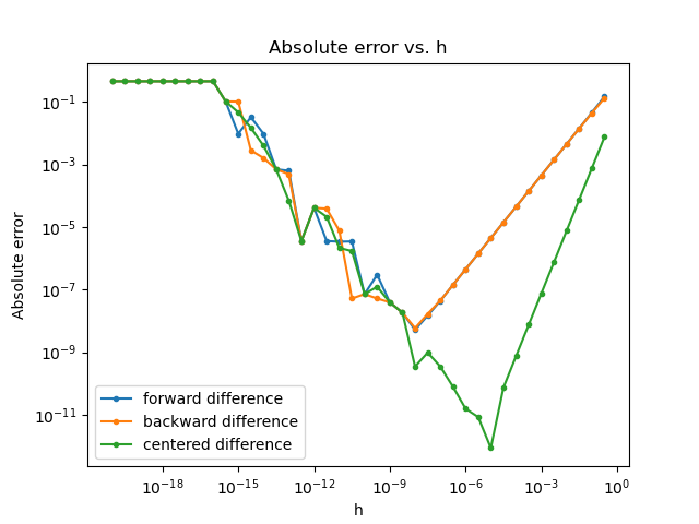
These formulas suggest that we can improve the approximation by making \(h\) arbitrarily small. Do we see this in practice? Consider \(f(x) = \sin (x)\) with a derivative evaluated at \(x = 20.24\). Applying these approximations,
import numpy as np
import matplotlib.pyplot as plt


def forward_difference(f, x, h):
    return (f(x + h) - f(x)) / h


def backward_difference(f, x, h):
    return (f(x) - f(x - h)) / h


def centered_difference(f, x, h):
    return (f(x + h) - f(x - h)) / (2 * h)


def plot_errors():
    x = 20.24
    f = np.sin
    f_prime = np.cos(x)
    h = 10 ** np.arange(-20, 0, 0.5)
    forward_err = np.abs(f_prime - forward_difference(f, x, h))
    backward_err = np.abs(f_prime - backward_difference(f, x, h))
    centered_err = np.abs(f_prime - centered_difference(f, x, h))

    fig, ax = plt.subplots()
    ax.plot(h, forward_err, marker='o', markersize=3, label='forward difference')
    ax.plot(h, backward_err, marker='o', markersize=3, label='backward difference')
    ax.plot(h, centered_err, marker='o', markersize=3, label='centered difference')
    ax.set_xscale('log')
    ax.set_yscale('log')
    ax.set_xlabel('h')
    ax.set_ylabel('Absolute error')
    plt.title('Absolute error vs. h')
    ax.legend()
    plt.show()

if __name__ == '__main__':
    plot_errors()

This is interesting! We see that our absolute errors initially decrease as \(h\) decreases, with orders reflective of the methods used. However, the errors eventually reach inflection points and then start to increase. This is due to the fact that our absolute error is actually composed of two types of error:
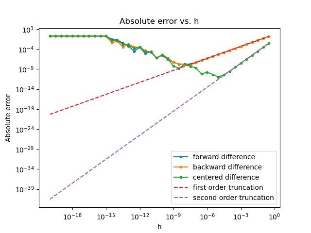
\[\text{absolute error} = \text{truncation error} + \text{roundoff error}.\]Roundoff error arises due to catastrophic cancellation in the numerator of these methods. We’ll discuss this shortly. To better delineate these errors, let’s add two dashed lines to the plot to indicate what our absolute error would be without roundoff error.
def plot_errors():
    ...
    first_order_truncation_err = f(x) / 2 * h
    second_order_truncation_err = f_prime / 6 * h ** 2
    ...
    ax.plot(h, first_order_truncation_err, '--', label='first order truncation')
    ax.plot(h, second_order_truncation_err, '--', label='second order truncation')
    ...

That’s quite a difference. Empirically, we see that truncation error initially dominates roundoff error. Only later, when the truncation error becomes very small, does roundoff error start to dominate. In fact, the roundoff error increases as \(h\) decreases. Therefore, these approximations are ill-conditioned.
Roundoff Error and Catastrophic Cancellation
Wikipedia defines catastrophic cancellation as
the phenomenon that subtracting good approximations to two nearby numbers may yield a very bad approximation to the difference of the original numbers.
To see this, let \(x, y \in \mathbb{R}\) with approximations \(\tilde{x}\) and \(\tilde{y}\), respectively. Assume \(x \approx y\). By the reverse triangle inequality,
\[\begin{align} |(\tilde{x} - \tilde{y}) - (x - y)| &= |(\tilde{x} - x) - (\tilde{y} - y)| \\ &\geq ||\tilde{x} - x| - |\tilde{y} - y|| \end{align}\]and so the relative error has a lower bound:
\[\frac{|(\tilde{x} - \tilde{y}) - (x - y)|}{|x - y|} \geq \frac{||\tilde{x} - x| - |\tilde{y} - y||}{|x - y|}\]The numerator of the bound could be small as it depends only on how well we’ve approximated \(x\) and \(y\). However, the denominator can also be very small if \(x \approx y\), and so the relative error can be arbitrarily large. In other words, subtraction is ill-conditioned at nearby inputs.
The important takeaway here is that catastrophic cancellation is inherent to subtraction itself, and present even if the difference is computed exactly. It’s why numerical libraries sometimes go to great lengths to avoid subtraction, and offer specialized methods to compute certain functions. For example, see Numpy’s expm1. To further analyze the effect of subtractive cancellation in the problem at hand, and determine values of \(h\) that minimize both types of error, we’ll have to discuss our specific approximation.
IEEE 754
In this case, we’re approximating real numbers using a finite precision representation. Specifically, NumPy’s float64
type uses the IEEE 754 double-precision binary floating-point format,
officially called binary64 (also known as double). A short exposé of this format will be helpful.

In binary64, as the name suggests, we represent real values in 64 bits of computer memory. Those 64 bits have the format pictured above. Let \(b_{i}\) denote the \(i\)th bit, for \(i \in \{0, 1, ..., 63\}\). Then, ignoring some special cases (e.g. NaN, Inf), the real value assumed by a 64-bit datum in this format is
\[(-1)^{\text{sign}}\underbrace{(1.b_{51}b_{50}...b_0)_2}_{\text{significand}} \times 2^{e - 1023}\]where \(e = (b_{62}b_{61}...b_{52})_2\). You can find a few examples of the translation on this Wiki page, or play around with this Python snippet:
def to_binary64_format(num):
    int64bits = np.float64(num).view(np.int64)
    return f'{int64bits:064b}'


def from_binary64_format(num):
    return np.int64(int(num, 2)).view(np.float64)


binary_64_format = to_binary64_format(20.24)
print(f'binary64: {binary_64_format}')
original_val = from_binary64_format(binary_64_format)
print(f'float64: {original_val}')
binary64: 0100000000110100001111010111000010100011110101110000101000111101 float64: 20.24
Machine Epsilon
Of course, we can’t represent an infinite set of values with a finite set of bits. Therefore, IEEE 754 defines a set of rules that dictate how a number \(x\) is rounded to the nearest representable one in binary64, denoted \(\text{fl}(x)\). We call \(\text{fl}(x)\) the floating point representation of \(x\). Going forward, we’ll use the notation \(\tilde{x}\) to mean \(\text{fl}(x)\) for simplicity.
Naturally, we’re interested to know the error in the representation of \(x\) by \(\tilde{x}\). As it turns out, we have a bound on the relative error of this representation:
\[\frac{|\tilde{x} - x|}{|x|} \leq \epsilon\]where \(\epsilon\) is known as interval machine epsilon. \(\epsilon\) is equal to the distance between 1 and the next smallest representable number larger than 1.0. In other words, the value of the unit in the last place (aka ulp) relative to 1. For binary64, that means \(\epsilon = 2^{-(p - 1)} = 2^{-(53 - 1)} = 2^{-52} \approx 2.2 \cdot 10^{-16}\), where the precision \(p = 53\) is the number of digits in the significand (including the leading implicit bit) in our binary64 representation. This is confirmed with some calls to NumPy’s finfo:
print((
    f'Number of bits in mantissa: {np.finfo(float).nmant}\n'
    f'Interval machine epsilon: {np.finfo(float).eps}'
))
Number of bits in mantissa: 52
Interval machine epsilon: 2.220446049250313e-16
Python’s math module also has a nice built-in for this:
print(math.ulp(1))
2.220446049250313e-16
This bound is independent of the type of rounding used. However, we can do better assuming that “round-to-nearest” is used:
\[\frac{|\tilde{x} - x|}{|x|} \leq \frac{\epsilon}{2} = u\]where \(u\) is known as rounding machine epsilon (also unit roundoff). You can find the derivation of this bound here. For binary64, \(p = 53\) and so
\[\begin{align} u &= \frac{\epsilon}{2} \\ &= \frac{2^{-(p - 1)}}{2} \\ &= 2^{-p} \\ &= 2^{-53} \\ &\approx 1.1 \cdot 10^{-16}. \end{align}\]Indeed, round-to-nearest is used by binary64 (and other double types) by default. For the rest of the article, when I say “machine epsilon,” I’m referring to this variant. Interestingly, IEEE 754 also requires exact (aka correct) rounding, meaning that the result of an arithmetic operation must be the same as if the operation were computed exactly and then the result rounded to the nearest floating point number. This guarantees that the relative error in each arithmetic operation is also bounded by \(u\).
Choosing the Step Size
Let’s perform some analysis to find a step size \(h\) that minimizes the combination of these two errors (truncation and roundoff) for each of the algorithms we discussed. We’ll discover that \(h\) is well-above machine epsilon in all cases.
Forward / Backward Difference
Define
\[g(x) = \frac{f(x + h) - f(x)}{h}.\]Then,
\[\begin{align} |f'(x) - \widetilde{g(x)}| &= |f'(x) - g(x) + g(x) - \widetilde{g(x)}| \\ &\leq \underbrace{|f'(x) - g(x)|}_{\text{truncation error}} + \underbrace{|g(x) - \widetilde{g(x)}|}_{\text{roundoff error}}. && \text{triangle inequality} \end{align}\]From before, we know that the truncation error is
\[h\frac{f^{''}(\xi)}{2}\]for some \(\xi \in [x, x + h]\). Define
\[M = \underset{x\in [x, x+h]}{\sup} |f''(x)|\]so that our truncation error can be written
\[\frac{Mh}{2}.\]Now, let’s bound our roundoff error. Recall that machine epsilon \(u\) provides a bound on the relative error of a floating point representation:
\[\frac{|\tilde{x} - x|}{|x|} \leq u.\]This will be handy shortly. Now, ignoring the errors generated in basic arithmetic operations, we have that
\[\begin{align} |\widetilde{g(x)} - g(x)| &= |\frac{\widetilde{f(x + h)} - \widetilde{f(x)}}{h} - \frac{f(x + h) - f(x)}{h}| \\ &= \frac{1}{h}|\widetilde{f(x + h)} - f(x + h) + f(x) - \widetilde{f(x)}| \\ &\leq \frac{1}{h}[|\widetilde{f(x + h)} - f(x + h)| + |f(x) - \widetilde{f(x)}|] && \text{triangle inequality} \\ &= \frac{1}{h}[|\widetilde{f(x + h)} - f(x + h)| + |\widetilde{f(x)} - f(x)|] \\ &\leq \frac{1}{h}[|f(x + h)|u + |f(x)|u] && \text{def. of machine epsilon} \\ &= \frac{u}{h}[|f(x + h)| + |f(x)|] \\ &= \frac{2u|f(x)|}{h}. && \text{assume $f(x) \approx f(x + h$)} \end{align}\]Now, define
\[L = \underset{x\in [x, x+h]}{\sup} |f(x)|\]so that we can write our bound as
\[\begin{align} \frac{2uL}{h}. \end{align}\]Therefore, we finally have that
\[\begin{align} |f'(x) - \widetilde{g(x)}| &\leq \frac{Mh}{2} + \frac{2uL}{h}. \end{align}\]We can find the optimal \(h\) (let’s call it \(h^*\)) by finding the critical point of our bound:
\[\begin{align} \frac{\partial}{\partial h}[\frac{Mh}{2} + \frac{2uL}{h}] &= 0 \\ \frac{M}{2} - \frac{2uL}{h^2} &= 0 \\ \frac{M}{2} &= \frac{2uL}{h^2} \\ h^2 &= \frac{4uL}{M} \\ h &= 2\sqrt{\frac{uL}{M}}. \end{align}\]If we plug this choice of \(h\) back into our bound on the absolute error, we have that
\[\begin{align} \frac{Mh}{2} + \frac{2uL}{h} &= \frac{2\sqrt{\frac{uL}{M}}M}{2} + \frac{2uL}{2\sqrt{\frac{uL}{M}}} \\ &= 2\sqrt{uLM}. \end{align}\]This is on order of \(\sqrt{u} \approx 10^{-8}\), meaning that forward difference with an optimal step-size only provides up to 8 digits of significant figures.
In practice, we usually don’t know \(M\) or \(L\), and so one rule of thumb is to use
\[h^* = \max(|x|, 1) \sqrt{u}.\]Centered Difference
The analysis here is the same as above, except that
\[\begin{align} g(x) = \frac{f(x + h) - f(x - h)}{2h} \end{align}\]and the truncation error is bounded by
\[\begin{align} h^2 \frac{f^{(3)}(\xi)}{6} \end{align}\]for some \(\xi \in [x - h, x + h]\). Now, define
\[S = \underset{x\in [x - h, x + h]}{\sup} |f^{(3)}(x)|\]so that the bound on the truncation error can be written
\[\begin{align} \frac{Sh^2}{6}. \end{align}\]Then, we have that
\[\begin{align} |f'(x) - g(x)| \leq \frac{Sh^2}{6} + \frac{2uL}{h}. \end{align}\]As before, we can find \(h^*\) by finding the critical point:
\[\begin{align} \frac{\partial}{\partial h}[\frac{Sh^2}{6} + \frac{2uL}{h}] &= 0 \\ \frac{Sh}{3} - \frac{2uL}{h^2} &= 0 \\ \frac{Sh}{3} &= \frac{2uL}{h^2} \\ h^3 &= \frac{6uL}{S} \\ h &= \sqrt[3]{\frac{6uL}{S}}. \end{align}\]Plugging back into our bound on the absolute error of this approximation, we have that
\[\begin{align} \frac{Sh^2}{6} + \frac{2uL}{h} &= \frac{S(\sqrt[3]{\frac{6uL}{S}})^2}{6} + \frac{2uL}{\sqrt[3]{\frac{6uL}{S}}} \\ &= (\frac{9SL^2}{2})^{1/3}u^{2/3}. \end{align}\]This is on the order of \(u^{2/3} \approx 10^{-11}\), meaning that centered difference with an optimal step-size provides up to 11 digits of significant figures.
Roundoff Error from Step
Of course, we can’t forget that there’s also roundoff error present in x + h. We can write this as \(x + h + \epsilon\) where \(\epsilon\) is our roundoff error. Then, our forward difference is really
\[\begin{align} \frac{f(x + h + \epsilon) - f(x)}{h} &= \frac{f(x + h + \epsilon) - f(x + h)}{\epsilon}\frac{\epsilon}{h} + \frac{f(x + h) - f(x)}{h} \\ &\approx f'(x + h)\frac{\epsilon}{h} + f'(x) && \text{def. of forward difference} \\ &\approx (1 + \frac{\epsilon}{h})f'(x). && \text{assume } f'(x+h) \approx f'(x) \end{align}\]Thus, if \(\epsilon\) is order \(u\) and \(h\) is order \(\sqrt{u}\) then we’ve added a relative error of order \(\sqrt{u}\) into the calculation. Therefore, to avoid this problem we usually define \(h\) (for first order methods) as
\[\begin{align} x_h &= x + h \\ h &= x_h - x \end{align}\]to ensure \(x + h\) and \(x\) differ by an exactly representable number.
Analysis
Let’s revisit the example we used to illustrate the issue with vanilla finite difference methods, where we considered \(f(x) = \sin (x)\). Specifically, let’s see if our derivations above align with the behavior we observed in practice. For forward / backward difference, we have \(L = 1\) and \(M = 1\), so
\[\begin{align} h^* &= 2 \sqrt{\frac{uL}{M}} \\ &= 2 \sqrt{u}. \end{align}\]For centered difference, \(S = 1\), so
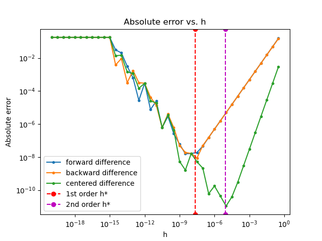
\[\begin{align} h^* &= \sqrt[3]{\frac{6uL}{S}} \\ &= \sqrt[3]{6u}. \end{align}\]Plotting these values of \(h\) on our original graph,
def plot_errors():
    ...
    u = np.finfo(float).eps / 2
    first_order_h = 2 * np.sqrt(u)
    ax.axvline(x=first_order_h, marker='o', linestyle='--', label='1st order h*', color='r')
    second_order_h = np.cbrt(6 * u)
    ax.axvline(x=second_order_h, marker='o', linestyle='--', label='2nd order h*', color='m')
    ...

we see that our choices of \(h\) are indeed optimal. Nevertheless, choosing the proper step size \(h\) is a careful art, requiring some analysis based on the function \(f\). Moreover, our accuracy is not close to machine epsilon. Can we do better? It turns out, yes! At least for a certain class of well-behaved functions, which includes \(\sin(x)\).
Complex Step Differentiation
Let’s assume that our function \(f\) is holomorphic at the point \(x\), but still mapping \(\mathbb{R} \to \mathbb{R}\).
Holomorphic Function
A function \( f: \mathbb{C} \to \mathbb{C} \) is holomorphic at a point \( a \in \mathbb{C} \) if it is differentiable at every point within some open disk centered at \( a \).
Complex Analytic Function
A function \( f: \mathbb{C} \to \mathbb{C} \) is complex analytic at a point \( a \in \mathbb{C} \) if in some open disk centered at \( a \) it can be expanded as a convergent power series $$ f(z) = \sum _{n=0}^{\infty}c_n (z - a)^n $$ where \( c_n \in \mathbb{C} \) represents the coefficient of the \( n \)th term.
Famously, holomorphic functions are complex analytic, and vice versa.
And we know that Taylor’s theorem generalizes
to complex analytic functions. So, we can consider a Taylor
polynomial for \(f\) centered at \(x \in \mathbb{R}\) and evaluated at \(x + ih\), where \(i = \sqrt{-1}\) and \(h \in \mathbb{R}:\)
for some \(\xi \in D(x, x + ih)\) (a disk centered at \(x\) with radius \(x + ih\)). Taking the imaginary component of both sides,
\[\begin{align} \operatorname{Im}(f(x + ih)) = hf^{'}(x) - h^3 \frac{f^{(3)}(\xi)}{6} \end{align}\]and so
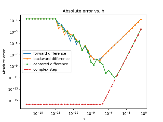
\[\begin{align} f^{'}(x) &= \frac{\operatorname{Im}(f(x + ih))}{h} + h^2\frac{f^{(3)}(\xi)}{6} \\ &= \frac{\operatorname{Im}(f(x + ih))}{h} + O(h^2) \\ &\approx \frac{\operatorname{Im}(f(x + ih))}{h}. \end{align}\]How cool! This approximation is known as the complex-step. Importantly, it’s a second-order method not subject to catastrophic cancellation. In other words, it doesn’t suffer from the roundoff error present in the other methods. That means we can take \(h\) arbitrarily small (e.g. \(10^{-200}\)) without worrying about roundoff error. To demonstrate, let’s update our code:
eps = np.finfo(float).eps


def complex_step(f, x, h):
    return np.imag(f(x + i * h)) / h


def plot_errors():
    ...
    complex_step_err = np.abs(f_prime - complex_step(f, x, h))
    # let's account for the subtractive cancellation introduced here, so the plot looks nice
    complex_step_err[complex_step_err < eps] = eps
    ...
    ax.plot(h, complex_step_err, linestyle='-.', marker='o', markersize=3, label='complex step')
    ...

Some Comments
- This method is typically slower than its finite difference counterparts, despite the fact that it only uses a single function evaluation. This is due to the expense of complex arithmetic. For example, a brief review of NumPy’s source (see here and here) suggests that we compute \(\sin(z)\) using the following identity: \(\sin(x + iy) = \cosh(y)\sin(x) + i \sinh(y)\cos(x)\). So we’re evaluating four trigonometric functions, instead of two. That’s, like, double the cost!
- As stated above, this method requires that \(f\) be complex analytic at the point we’re evaluating the derivative. To see where this can go wrong, consider \(f(z) = \\|z\\|^2\) where \(z = x + iy\) for some \(x, y \in \mathbb{R}\). Then, \(\\|z\\|^2 = x^2 + y^2\), and so \(f\) is a real-valued function. By the Cauchy-Reimann equations, we know that real-valued functions cannot be complex analytic unless they’re constant. \(f\) is not constant, and so it’s not complex analytic. Applying the complex step blindly would return \(f'(x) = 0\) everywhere, when we know that \(f'(x) = 2x\)!
- This method cannot be iterated to compute higher order derivatives, unlike finite differences. You might be tempted to compute \(f''(x)\) via \(f''(x) = \frac{\operatorname{Im}(f'(x + ih))}{h}\) and \(f'(x+ih) = \frac{\operatorname{Im}(f(x + 2ih))}{h}\). However, although \(f'(z)\) is analytic, this method can only be used to compute \(f'(z)\) for real arguments. So we cannot perform the first step of the iteration.
- There’s an exciting connection to forward-mode automatic differentiation (AD) via dual numbers which we won’t go into here (at least for now). You can read more about that here. However, we’ll note that the complex-step method is less efficient than forward-mode AD due to some unnecessary computations. That partly explains why you rarely see this method in practice.
- We also recover a second-order approximation to \(f\) for free, as \(\operatorname{Re}(f(x+ih)) \approx f(x)\).
Alternate Derivation
Suppose \(z \in \mathbb{C}\). Then, \(z = x + iy\) for some \(x, y \in \mathbb{R}\). For \(f: \mathbb{C} \to \mathbb{C}\), we have
\[\begin{align} f(z) &= f(x + iy) \\ &= u(x, y) + i v(x, y) \end{align}\]where \(u\) and \(v\) are real differentiable functions. For our purposes, we’re specifically interested in a function \(f\) that’s:
- Complex analytic at a point \(a \in \mathbb{R}\).
- Real-valued for real inputs.
If \(a \in \mathbb{R}\), i.e. \(y = 0\), then the second condition implies \(u(x, 0) = f(x)\) and \(v(x, 0) = 0\). By the first condition, we must satisfy the following at \(a\):
\[\begin{align} \frac{\partial u}{\partial x} &= \frac{\partial v}{\partial y} && \text{Cauchy-Reimann} \\ \frac{\partial u}{\partial x}|_{y=0} &= \frac{\partial v}{\partial y}|_{y=0} \\ \frac{\partial u(x, 0)}{\partial x} &= \lim_{h \to 0} \frac{v(x, h) - v(x, 0)}{h} && \text{limit definition of derivative at a point} \\ \frac{\partial f(x)}{\partial x} &= \lim_{h \to 0} \frac{v(x, h)}{h} && u(x, 0) = f(x) \text{ and } v(x, 0) = 0 \\ f'(x) &= \lim_{h \to 0} \frac{\operatorname{Im}(f(x + ih))}{h}. && v(x, h) = \operatorname{Im}(f(x + ih)) \end{align}\]